Predictive maintenance in six steps

Predictive maintenance: everyone talks about it and seems to know how to do it. But what is it really? Enos Postma takes us into the world of assets, predictive maintenance, statistics and algorithms and explains how to implement predictive maintenance in six clear steps. 

Why predictive maintenance?

Within the industry, we depend on the technical availability of many components; machines, systems and installations to, for example, transport, produce steel and supply gas. Traditionally, Stork as well as other companies have helped their customers keep production lines running according to an industry-proven Reliability Centered Maintenance (RCM) method. This is done through a combination of maintenance methods: reactive based maintenance (RBM), time-based maintenance (TBM) and condition-based maintenance (CBM). A disadvantage of way of working is that it is based on the mean time between failure (MTBF) and on the assumption that the pattern of failure increases over time. This means that because of the variation in MTBF, a condition-based strategy or a time-based strategy may lead to a component failure more often than one would like, resulting in lost production time and revenues and potentially unnecessarily replaced components.

Another scenario occurs when degradation is detected by performing maintenance inspections, resulting in an increase in man-hours and sometimes even a higher workload than in a run-to-failure scenario. Since only 18% of errors are age-related and 82% have an arbitrary failure pattern (NASA/US Navy, 2008, see Figure 1), RCM does not offer a complete solution for optimizing maintenance.

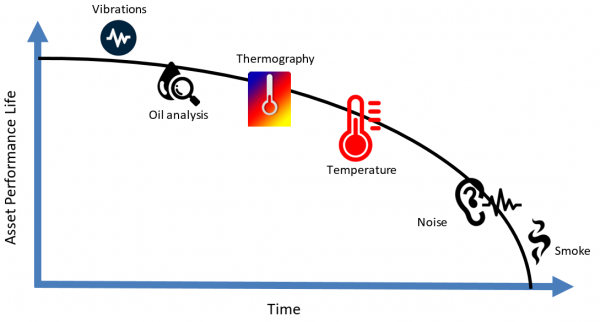
Figure 1

This is where the importance of predictive maintenance becomes clear. It is a means of optimizing the technical availability of an asset by influencing maintenance parameters such as frequency and the ongoing maintenance strategy. Methods and techniques for predictive maintenance are thus designed to help determine the condition (health) of assets in use: when is maintenance required?

How do you achieve this?

The question then is how to realize predictive maintenance. First, we add sensors to the system that monitor and collect operational performance data. At Stork, we see that many companies already have significant amounts of data that is used to control the processes. What is even better is that this historical data has often been stored in their historian systems for years. We advise clients to use this data actively in predicting the remaining useful life of assets. Typically, predictive maintenance data includes a timestamp, a series of sensor measurements collected at the same time with a timestamp and device identifiers.

The pf-curve in figure 2 below illustrates that an asset delivers a certain performance at time t = 0, and that this performance decreases as time goes by. This may be due to use, aging, wear and tear, environment and many more factors.

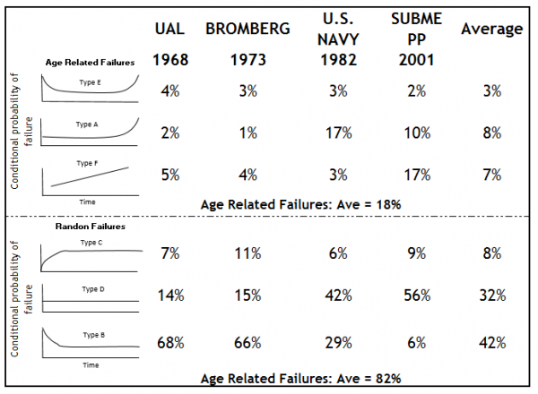
Figure 2

Figure 2 also illustrates that during the lifetime of an asset, you can create anomaly categories from the various types of data as the asset degrades over time. The first indication of degradation can result from vibration measurements and oil analysis. After that, the asset will show higher (than normal) temperature readings. It can be difficult to determine exactly when a failure mode has started, but we can look for signs of decay to address the problem before the asset fails. It is therefore important to understand the behavior of the sensor measurements for each failure mode of every asset.

From experience we know that classification and clustering algorithms best fit the application for predictive maintenance. These algorithms allow you to categorize historical data (asset behavior) into predefined classification / cluster groups. For example, the combination of an increase in temperature and a slight increase in the vibration measurement value results in a category label such as "A week before failure". Again, data categorization (labeling) is an important part of predictive maintenance. These labels are determined for each individual case (every combination of asset and failure mode) and may vary from a binary label such as "Good Performance" or "Poor Performance" to a more continuous classification for the remaining useful life "30 days", "29 days", etc. Algorithms that can be used for classification include (linear) Support Vector Machine, Naïve Bayes, KNeighbors and logistic regression, and for clustering these are KMean, MeanShift and SpectralCLustering. Which algorithms you choose for the best fit depends on the sample size, the data type (labeled, quantity or text data) and in-depth knowledge of the asset's failure modes.

Six-step model for asset performance managment

Stork has developed a six-step model that helps our customers choose the right algorithm and implementation method in your organization.

The first step is to understand the functionalities of the asset and the means of failure. Fault data is extracted from your Computerized Maintenance Management System (CMMS) and process data is extracted from the manufacturer's manual. The result of this phase is an in-depth understanding of the dominant failure mode and its (financial) impact on the organization.

The second step involves selecting historical data containing data streams or patterns that can be labeled as "good performance" or "poor performance". Since algorithms can only learn patterns that are already present in the data, the target set must be large enough to contain these patterns, while still remaining concise enough to be found within an acceptable time frame. The data sets are often stored in different databases that require additional integration. In addition to the quantity, the quality of the data is also assessed during this phase. All data sets must have the same timestamp to be able to use multiple sensors for one prediction. Interpolation is then applied for missing data and noise data is removed.

The third step (modeling) is to extract patterns from the data. This includes the selection and application of suitable (mathematical) algorithms and the development of a model that describes the pattern. This step is often accompanied by "traditional" statistical analysis, data visualization and simulation of historical data (development of demo version).

In the fourth step, a business case is developed to substantiate the benefits of predicting a failure mode. The costs of writing an algorithm and real-time monitoring are compared with the financial benefits. Potential savings can be divided into two main forms: (1) Prevent or minimize production downtime and (2) Optimize periodic maintenance work. Other benefits include the capitalization of knowledge, extending the life of assets, as well as improvements in health, safety and the environment. These "other" benefits are not always present and if they are, it can be difficult to quantify them.

If the business case has a positive result, you can proceed to the implementation phase (step 5) by carrying out the actions defined in the previous phases. The result of this phase is that the organization is able to use the information provided by the model to eventually adjust maintenance intervals and work processes.

Finally, as a sixth and final step, the improvement cycle must be closed. During the operational phase, the algorithm begins to be a self-learning model due to continuous improvement by the Data Scientist. Additional error patterns are continuously added to the algorithm.

Due to the large amount of data already available and the ability to easily develop complex algorithms, now is the time to use it in order to predict the health of our most important assets. The development of effective algorithms for predictive maintenance takes time and payment of learning fees is inevitable. However, I am convinced that the overall benefits far outweigh the initial investment.

Type I And Type II Errors In Predictive Maintenance Two types of errors can occur in statistics. The Type I error is the incorrect rejection of a correct null hypothesis (also known as an "error positive" finding), while a Type II error incorrectly endorses a false null hypothesis (also known as an "error negative" finding). This is also an issue in predictive maintenance. The error corresponding to the type I error is that you detect an asset that does not work, but that the performance of the asset is actually good (healthy). This error gives an incorrect justification for investing in predictive maintenance. This will lead to a technician being mobilized to control the asset while it is in good condition or, even worse, you replacing components of a perfectly healthy asset. That's why I believe that the maintenance and reliability engineers of the Industry 4.0 era can call themselves experts when they discover tomorrow why the things they predicted yesterday didn't happen. The Type II error has more implications in terms of costs. In this case, an error occurred but was not predicted. Both errors are prevented by setting up an improvement process (step 6 of our APM model). This means that algorithms must constantly learn new patterns of failure until the algorithm is smart enough to correctly predict 100% of the failing assets.